(三十五)训练曲线、预测散点与混淆矩阵
1. 读取普通历史记录画曲线
# 项目文件:training_project/src/readingtorch/plots.py
import argparse
import json
from pathlib import Path

import matplotlib

import numpy as np
import torch

from .checkpoint import load_checkpoint
from .data import read_raw
from .predict import Predictor

matplotlib.use("Agg")  # 直接输出文件,命令行运行不需要打开绘图窗口。
import matplotlib.pyplot as plt  # noqa: E402

plt.rcParams.update(
    {
        "font.family": "Microsoft YaHei",
        "axes.unicode_minus": False,
        "figure.facecolor": "#F5F7FB",
        "axes.facecolor": "white",
        "text.color": "#24324A",
        "axes.labelcolor": "#24324A",
    }
)


def plot_run(folder, data):
    folder = Path(folder)
    report = json.loads((folder / "history.json").read_text(encoding="utf-8"))
    history = report["history"]
    fig, ax = plt.subplots(figsize=(8, 4.6), layout="constrained")
    ax.plot(
        [r["epoch"] for r in history],
        [r["train"]["loss"] for r in history],
        label="训练损失",
        color="#4657B5",
    )
    ax.plot(
        [r["epoch"] for r in history],
        [r["val"]["loss"] for r in history],
        label="验证损失",
        color="#087F82",
    )
    ax.axvline(report["best_epoch"], color="#A85D11", linestyle="--", label="选中轮数")
    if all(row["train"]["loss"] > 0 and row["val"]["loss"] > 0 for row in history):
        ax.set_yscale("log")  # 把后期较小的损失变化一起展开。
    ax.set(
        xlabel="完成轮数",
        ylabel="平均损失(本图为对数刻度)" if ax.get_yscale() == "log" else "平均损失",
        title="回归训练" if report["task"] == "regression" else "图形分类训练",
    )
    ax.legend()
    ax.grid(alpha=0.18)
    fig.savefig(folder / "loss.png", dpi=180, bbox_inches="tight", pad_inches=0.15)
    plt.close(fig)
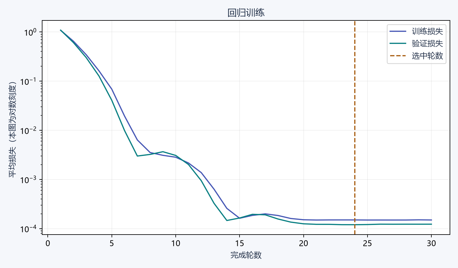
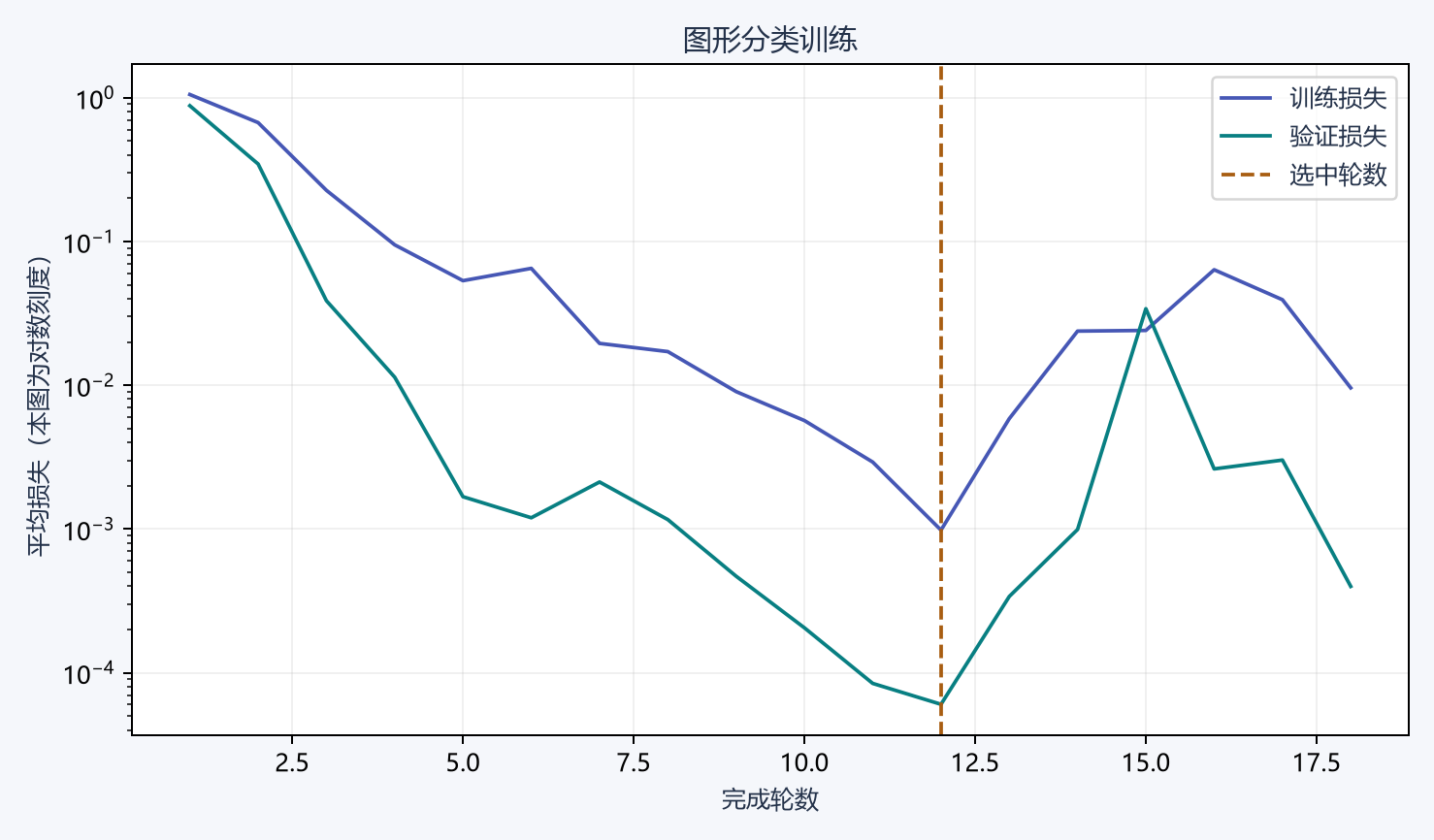
横轴是已经完成的轮数,纵轴是相应平均损失。这次曲线使用对数刻度,让从一左右下降到万分之一附近的变化都能展开;纵轴相同距离表示相同比例的变化。训练曲线来自每批更新前取得的损失,验证曲线来自该轮结束后的固定模型,因此二者的采样时刻也要一起理解。虚线标出验证集选中的轮数。
# 续写同一文件:training_project/src/readingtorch/plots.py
    # 已选定的模型和保存的测试编号一起用于结果图。
    predictor = Predictor(folder / "best.pt")
    saved = load_checkpoint(folder / "best.pt")
    x, y = read_raw(report["task"], Path(data))
    ids = saved["splits"]["test"]
2. 用测试样本检查预测分布
# 续写同一文件:training_project/src/readingtorch/plots.py
    # 测试集预测在模型选择完成后读取,分别用散点和计数矩阵表达。
    if report["task"] == "regression":
        prediction = [predictor.pages(*x[index].tolist()) for index in ids]
        actual = y[ids, 0].tolist()
        fig, ax = plt.subplots(figsize=(6.5, 5), layout="constrained")
        ax.scatter(actual, prediction, color="#087F82", s=30, label="测试样本")
        ax.plot(
            [min(actual), max(actual)],
            [min(actual), max(actual)],
            "--",
            color="#A85D11",
            label="预测等于实际",
        )
        ax.set(xlabel="实际页数", ylabel="预测页数", title="回归模型的 48 条测试记录")
        ax.legend()
    else:
        confusion = np.zeros((3, 3), dtype=int)
        with torch.inference_mode():
            predicted = predictor.model(x[ids]).argmax(1)
        for true, guess in zip(y[ids], predicted):
            confusion[int(true), int(guess)] += 1
        fig, ax = plt.subplots(figsize=(6.5, 5), layout="constrained")
        ax.imshow(confusion, cmap="GnBu")
        for row in range(3):
            for column in range(3):
                ax.text(
                    column,
                    row,
                    str(confusion[row, column]),
                    ha="center",
                    va="center",
                    fontsize=18,
                    color="white"
                    if confusion[row, column] > confusion.max() / 2
                    else "#24324A",
                )
        ax.set(
            xticks=range(3),
            yticks=range(3),
            xticklabels=saved["classes"],
            yticklabels=saved["classes"],
            xlabel="预测类别",
            ylabel="实际类别",
            title="72 张测试图的混淆矩阵",
        )
    fig.savefig(folder / "test.png", dpi=180, bbox_inches="tight", pad_inches=0.15)
    plt.close(fig)
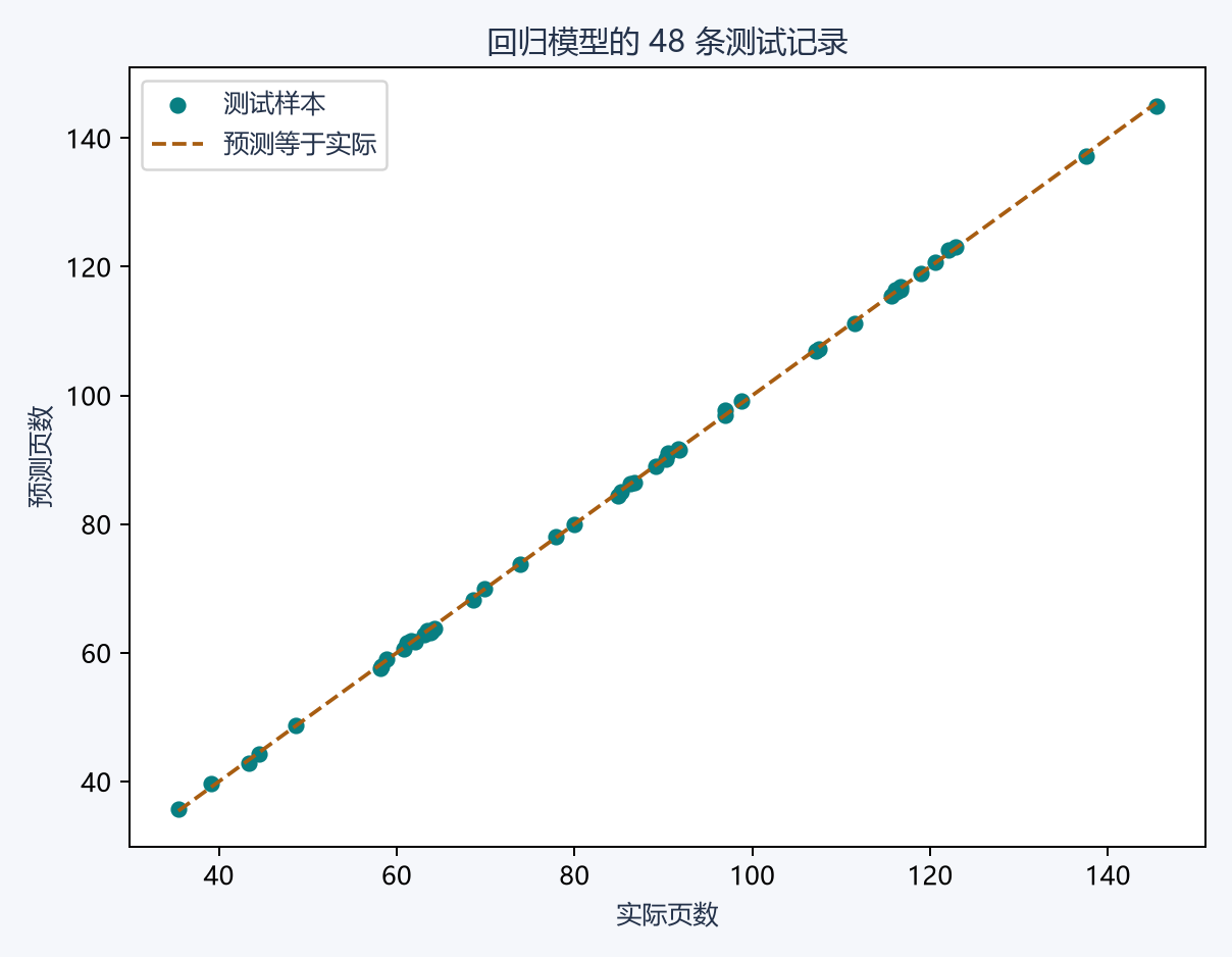
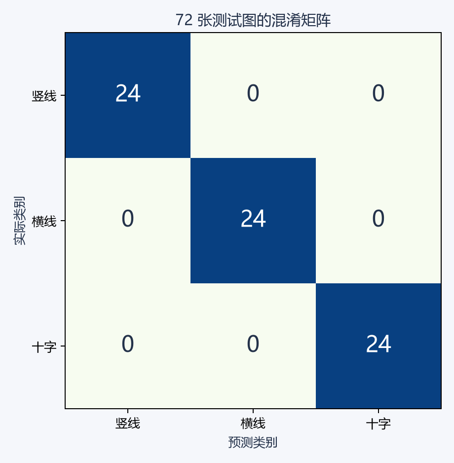
回归图把实际页数放在横轴、预测页数放在纵轴;靠近“预测等于实际”的虚线表示误差较小。分类的混淆矩阵以行表示实际类别、列表示预测类别,每个格子统计落在该组合的张数,主对角线是判断正确的样本。
# 续写同一文件:training_project/src/readingtorch/plots.py
def main():
    # 图表入口接收训练输出目录与对应数据文件。
    parser = argparse.ArgumentParser(description="绘制一次训练的曲线与测试结果")
    parser.add_argument("folder")
    parser.add_argument("--data", required=True)
    args = parser.parse_args()
    plot_run(args.folder, args.data)


if __name__ == "__main__":
    main()
# 从训练输出与原数据生成曲线和测试图,不重新训练。
uv run python -m readingtorch.plots runs/regression --data data/reading.csv
uv run python -m readingtorch.plots runs/images --data data/symbols.npz